Mastering Six Sigma Standard Deviation: Calculations, Analysis, and Process Improvements

In today’s highly competitive business landscape, organizations must continually strive to improve the quality and efficiency of their processes to satisfy customers and stay ahead.

This is where Six Sigma – a rigorous methodology focused on reducing defects and variability – can make an immense difference.

At the very core of the Six Sigma methodology lies an essential statistical concept known as standard deviation.

Standard deviation forms the backbone for data analysis and fact-based decision-making in the Six Sigma approach.

By quantifying the amount of variability or dispersion in a process, standard deviation enables Six Sigma practitioners to pinpoint quality issues, identify risks, and implement targeted solutions.

Mastering standard deviation is key to executing Six Sigma initiatives successfully and driving sustained process improvements over time.

What is Six Sigma Standard Deviation?

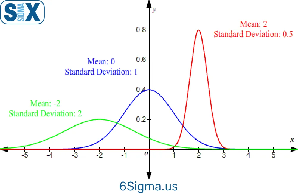
Standard deviation is a statistical measurement used in Six Sigma to determine the variation in a process. It measures how far each data point deviates from the mean or average.

In simple terms, standard deviation quantifies the dispersion or spread of data in a dataset. A process with a high standard deviation will have largely varying outputs, while a process with a low standard deviation will generate relatively consistent outputs.

Definition and Meaning of Standard Deviation

The standard deviation formula measures the average distance between each data point and the mean. The larger the standard deviation, the more variability in the process.

Mathematically, standard deviation is calculated by taking the square root of the variance or average of squared deviations from the mean.

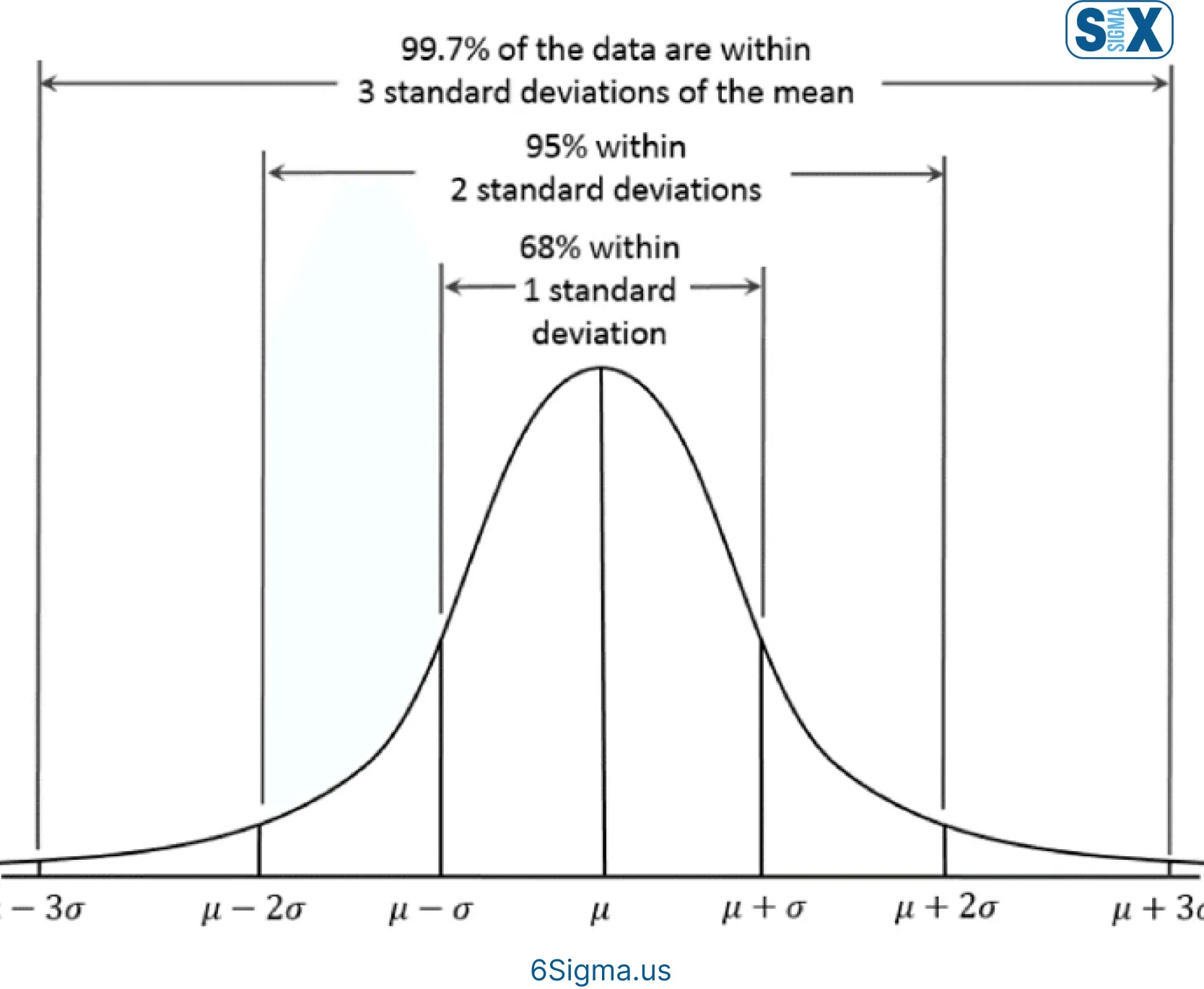
The concept of standard deviation is inextricably linked to the normal distribution or bell curve used in statistics.

In a normal distribution, 68% of data points fall within +/- 1 standard deviation from the mean, 95% within +/- 2 standard deviations, and 99.7% within +/- 3 standard deviations. Six Sigma aims for accuracy up to six standard deviations, hence the methodology’s name.

Role in Six Sigma Methodology

As a key metric in statistical analysis, standard deviation allows Six Sigma practitioners to determine the stability and precision of critical processes. It plays an instrumental role within Six Sigma’s define-measure-analyze-improve-control (DMAIC) approach to process improvement.

During the ‘measure’ phase, standard deviation helps identify process variation and potential causes.

The ‘analyze’ phase helps pinpoint sources of variation via methods like ANOVA and regression analysis. During ‘improve’ and ‘control’, reducing standard deviation helps enhance process capability and control fluctuations.

Relation to Process Improvement

While processes have common cause variation, special causes also introduce unpredictability. By tracking standard deviation over time using control charts, abnormal points and trends become visible.

This allows Six Sigma teams to isolate special causes and create solutions to minimize variation and defects.

The higher the sigma level (lower the standard deviation), the better the process performance.

Decreasing variation improves quality, reduces waste, lowers costs, and boosts customer satisfaction – all integral aspects of process improvement.

For instance, according to Gartner, 95% of the 150 BPM (Business Process Management) initiatives have been effective.

Calculating Six Sigma Standard Deviation

Understanding how to calculate standard deviation by hand and using tools is essential for Six Sigma practitioners to analyze process data.

We will cover the key formulas, tools, and a step-by-step calculation example.

Formulas for Population vs Sample Data

Two formulas exist for standard deviation – one for population data, and another for sample data extracted from a population.

Population Standard Deviation Formula:

σ = √∑(x – μ)² / N

Sample Standard Deviation Formula:

s = √∑(x – x̄)² / (N – 1)

Here, σ refers to the population standard deviation, s is the sample standard deviation, x is the value of each data point, μ and x̄ are the population and sample mean respectively, and N is the total number of data points.

It’s vital to use the appropriate formula based on whether complete population data is available or a sample is being analyzed.

Tools for Calculation

While manual calculation is useful for understanding, Six Sigma projects often rely on software tools for calculating standard deviation:

• Minitab
• Microsoft Excel using the STDEV formulas
• Statistical programming languages like R and Python
• Online calculators for quick, one-off deviation checks

Leveraging such tools reduces effort and the risk of human error during statistical analysis.

Step-by-Step Manual Calculation

Let’s take an example dataset and walk through the step-by-step process manually:

Dataset = {2, 4, 6, 8, 10}

1. Calculate the Mean – Sum of all data points divided by count
   
   Here, Mean = (2 + 4 + 6 + 8 + 10)/5 = 6
   
2. Determine the deviations from the Mean for each point
   
   Deviations = {-4, -2, 0, 2, 4}
   
3. Square the deviations
   
   Squared Deviations = {16, 4, 0, 4, 16}
   
4. Calculate the Average Squared Deviation = Sum of Squared Deviations/Count
   
   Here, Average Squared Deviation = 40/5 = 8
   
5. Take the square root of the Average Squared Deviation to get the sample standard deviation.
   
   Here, Sample Standard Deviation = √8 = 2.83

By following this step-by-step approach, both population and sample standard deviation can be calculated manually.

Interpreting Six Sigma Standard Deviation

While calculating standard deviation is important, interpreting its implications is vital for process enhancements. We explore key insights and applications below.

Small vs Large Standard Deviations

The absolute standard deviation value offers clues into process stability:

• Smaller deviation signals output largely conforming to the average
• Larger deviation indicates unpredictable, fluctuating outputs

For example, a process with a standard deviation of 1 mm suggests products mostly vary in size by 1 mm. One with a 5 mm deviation will have more variable sizes.

Over time, reduced standard deviation implies improving process control and capability.

Impact of Standard Deviation on Process Variability and Quality

The higher the output variability, the lower the process quality and customer satisfaction. Products well outside specifications lead to defects and rework.

For instance, chemical formulations deviating in ingredient proportions can detrimentally impact quality and user safety. In manufacturing, unacceptable dimensional variations lead to scrapped items.

Since standard deviation quantifies variability, it is inextricably tied to quality levels.

Using Standard Deviation Analysis to Identify Improvements

Analyzing deviation trends helps pinpoint improvement areas, like:

• Operator training needs – unusually high deviations signal a lack of skill
• Defective equipment – consistent deviations point to improperly calibrated machines
• Substandard materials – component deviations translate to output deviations

Comparing deviations across product batches, machines, operators, etc. reveals problem sources. Addressing these persistently high deviations via root cause analysis and corrective actions leads to superior stability.

Six Sigma Standard Deviation in Practice

While a theoretical concept, standard deviation has manifold real-world applications within the Six Sigma approach for driving process enhancements.

Application in Statistical Process Control (SPC)

Statistical process control (SPC) leverages data analytics for quality monitoring. Control charts help differentiate between common and special cause variations.

The two most commonly used control charts – Xbar-R and Xbar-S plot the mean and standard deviation for subgroups of data points. By visualizing deviation trends, out-of-control conditions requiring investigation become apparent.

As the process stabilizes, the standard deviation inconsistencies reduce over time. This signals improved predictability and minimal special causes influencing output.

Control Charts and Monitoring Process Performance

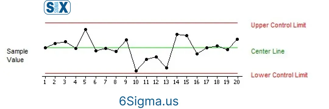
The central line in a control chart represents the overall process mean while the upper and lower control limits (UCL and LCL) are based on standard deviation. Typically UCL and LCL are set at ±3 standard deviations from the mean.

Data points beyond these control limits indicate statistically significant deviations warranting corrective action. Frequently, this signals the introduction of an unexpected special cause into the system.

Observing standard deviation patterns over time on control charts provides a snapshot of process stability and consistency.

Capability Analysis to Meet Specifications

While control charts utilize standard deviation to monitor stability, capability indices use it to assess process performance against requirements.

Key metrics like Cp and Cpk rely on minimum, maximum, and standard deviation measurements to determine process spread. By generating these indices, organizations quantify their ability to meet tolerances and identify improvement opportunities.

For Six Sigma teams, these actionable insights translate to targeted solutions that enhance output precision, reduce deviations, and boost quality.

Forrester reports that BPM Statistics initiatives can yield up to 30-50% improvement in productivity.

Case Study: Reducing Deviation in Television Assembly

A leading television manufacturer was facing complaints regarding inconsistent screen sizes for their latest 43-inch model. While the technical specification called for a 42.5-inch to 43.5-inch diagonal length, finished products were exhibiting higher variability.

A Six Sigma project team was tasked with investigating and reducing standard deviation in the screen assembly process.

Measure Phase

The team started by collecting screen diagonal size data for 100 recently assembled television sets. The average screen size came to 43.1 inches.

However, the standard deviation was found to be 0.8 inches – higher than desired.

On analyzing the data distribution and process steps, the primary source of variation was determined to be the manual placement of screens into plastic housing frames before final assembly.

Improve Phase

Multiple ideas were considered to control the positioning deviation caused during manual placement. Finally, the team decided to develop a specialized alignment jig with guides and markings. This optimized operator efficiency in centering the screen consistently, without consuming additional cycle time.

Results

A month after introducing the specialized jigs, the standard deviation of screen sizes reduced from 0.8 inches to 0.2 inches – a 75% improvement.

The number of customer complaints regarding screen size also lowered by 80%, directly enhancing brand reputation.

This case study illustrates how Six Sigma standard deviation analysis and statistical thinking catalyzed measurable improvements in a manufacturing process through data-driven problem-solving.

Common Mistakes and Challenges

While a vital Six Sigma tool, applying standard deviation incorrectly can severely impact analysis and decisions. We explore some key pitfalls to avoid.

Sample vs Population Data Issues

A common slip-up is using sample data formulas and inferences inaccurately for population datasets and vice versa.

By assuming incomplete sample data represents overall distribution or generalizing findings from a sample across populations blindly, erroneous conclusions get drawn.

Six Sigma teams must precisely identify whether a dataset constitutes the full population or a representative sample before analysis.

Thereafter, the appropriate formula and careful, contextual interpretations are critical.

Understanding Variation Origins

Carefully studying standard deviation trends provides clues to the origin of output variations. However, mechanically assuming higher deviation is automatically detrimental can sometimes backfire.

For example, a restaurant kitchen introduced automation to reduce human inconsistency in preparing raw potato fries for cooking.

This led to a lower standard deviation but customer complaints rose regarding soggy fries. Detailed investigation revealed that while automated cutting boosted size consistency, it also damaged starch granules more.

This caused higher moisture retention ultimately impairing taste and texture despite improving deviation metrics.

Thus, thoughtful analysis of causes and impacts is essential before pursuing deviations single-mindedly.

Predicted vs Empirical Standard Deviation

In project management approaches, standard deviation gets predicted early on using three-point estimates – best case, worst case, and most likely. This helps in planning budgets and timelines.

In Six Sigma, however, empirical, actual standard deviation calculated from real datasets takes precedence during analysis.

This quantifies true, demonstrable variation within a system. Relying solely on predictions risks masking pressing quality issues that surface during execution.

Therefore, while useful for forecasts, projected deviation measures cannot replace empirically derived observations and trends. Six Sigma teams must analyze genuine data mathematically firsthand.

Importance for Driving Process Improvements

While a statistical measure on the surface, standard deviation profoundly impacts operational enhancement initiatives in multifarious ways:

Robust Data Analysis: Standard deviation enables a detailed examination of process data – revealing vital aspects like stability, variability, and control. Instead of superficial reviews, Six Sigma teams can perform rigorous analytical evaluations leveraging deviation.

Targeted Solutions: Trends and hypotheses uncovered during analysis facilitate a nuanced, evidence-based path toward focused process improvements. Rather than blind guesses, standard deviation provides a beacon toward pinpointed solutions.

Prioritization: In large systems with hundreds of processes, organizations can numerically prioritize areas needing intervention based on deviation metrics. Worst performers ranked by highest standard deviations become natural starting points for improvement projects.

Ongoing Monitoring: Embedding standard deviation computation within regular reporting procedures sustains attention on critical processes. Any rising deviations signal potential degradation before issue amplification.

This keystone metric forms the very basis of statistical rigor that Six Sigma is renowned for across the global quality landscape today.

Key Takeaways

As we have seen, standard deviation contains invaluable insights for Six Sigma process excellence initiatives. Here are some crucial lessons to internalize:

• Standard deviation quantifies process variability and guides quality targets.
• Reducing deviation improves stability, capability and predicts long-term performance.
• Manual calculation provides intuitive understanding, software handles complex analysis.
• Control charts visualize variation, while capability indices evaluate specification readiness.
• Misusing sample vs population data distorts reality and misguides decisions.
• Employ with complementing metrics like mean and process capability indices.
• While chasing low deviation, maintain holistic process health based on all critical parameters.
• Keep evaluating multiple inputs to determine the root causes of variation.

In essence, standard deviation acts as an essential guidepost offering actionable inputs to boost process efficiency in a data-savvy manner.

However, teams must contextualize findings along with organizational needs. A balanced approach covering business priorities beyond purely statistical goals leads to genuine operational excellence – the core Six Sigma tenet.

Best Practices to Leverage Six Sigma Standard Deviation

To harness the potential of standard deviation for enhancing processes, Six Sigma practitioners should embrace these proven guidelines:

• Start by Quantifying Inherent Variation: Establish an overall variability benchmark early in DMAIC projects before further diagnostics. This identifies improvement scope.
• Analyze Trends not Just Absolute Values: While current deviation guides minimum goals, analyzing trends over time informs stabilization trajectories and control effectiveness.
• Bifurcate Data for Granularity: Where possible, slice data into meaningful subgroups to expose localized deviations. For instance, analyzing deviation shift-wise exposes intra-day patterns.
• Compare Multiple Metrics: Standard deviation alone cannot indicate health. Cross-tabulate deviation against defects rate, process capability index, cost of quality, and other metrics for comprehensive diagnostics.
• Revise Control Limits Accordingly: As improvement projects hit milestones, reconsider control limits based on updated, lower standard deviation values instead of historical levels.
• Sustain Gains with Process Controls: Support deviation reduction with statistical process controls to sustain achievements. This prevents backsliding over time after initial progress.

By inculcating these practical steps, Six Sigma teams can maximize leverage from standard deviation for enabling data-driven process enhancements in line with business objectives.