All About Normality Test in Statistical Analysis. Lean Six Sigma

In statistics, the assumption of normality test plays a big role in ensuring results make sense and can be relied on.

Many common tests like t-tests, ANOVA, and regression analyses assume data fits under a bell curve shape. Not meeting this assumption can lead to wrong conclusions and beliefs that can’t be trusted.

Normality tests are stat tools made to check if a dataset closely matches what’s expected in a normal distribution. They provide a clear measure of just how bell curve-like the numbers are.

It’s especially important to test normality when sample sizes are small. Even slight differences from normal then have a strong effect on analysis accuracy.

Additionally, many statistical methods are based on the central limit theory. This idea is that as more data is included, the average starts to look increasingly like a normal distribution shape.

Key Highlights

• Normality tests are stat tools that check if a set of numbers closely matches a normal bell curve shape. Determining normality is a key step for most common statistical exams.
• Popular normality tests include Shapiro-Wilk, Kolmogorov-Smirnov, Anderson-Darling, and visual methods like comparing data plots to a straight line.
• If the normal shape isn’t followed, it means test results and conclusions drawn from analyses could be wrong.
• The best normality test depends on sample size, extreme values, and planned statistical techniques.
• Checking normality is important in many fields like quality monitoring, finances, psychology and science research using stats. Not doing so risks inaccuracies in interpreting analyses.
• Normality testing provides assurance numbers fall as expected under that characteristic bell curve. This verification upholds the integrity of crucial statistical work across many domains.

What is the Normality Test?

Many common statistical tests assume data follows a bell curve shape, known as the normal distribution. Meeting this assumption is important, as failing it can produce misleading results and conclusions.

Normality tests let analysts determine if a dataset matches the normal shape well enough.

This distribution is symmetric like a bell and is used widely due to the theory stating sums or averages of independent random variables tend toward it regardless of the originals.

Checking normality is an important preprocessing and data exploration step. Breaking its assumption can impact the validity of techniques like t-tests, ANOVA, and regression that rely on it.

Non-normal data may cause inaccurate p-values, confidence intervals, and significance testing. Deviations from normality can happen due to:

• Skewed data with a long tail on one side
• Heavier or lighter tails than a bell curve
• Outlier extreme values outside typical ranges
• Uneven variance as other variables change

Normality tests provide an objective way to measure just how far from normal a set strays. This shows if the variance requires methods not relying on the normal shape.

Types of Normality Test

There are several statistical tests available to assess whether a dataset follows a normal distribution.

The choice of test depends on factors such as sample size, the underlying distribution, and the sensitivity required. Some common normality tests include:

Graphical Methods

• Normal Probability Plot: A graphical technique that plots the quantiles of the data against the quantiles of a normal distribution. If the data is normal, the points will follow an approximately straight line.
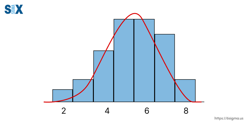
• Histogram with Overlaid Normal Curve: Visually comparing the shape of a histogram of the data to a normal distribution curve can give an initial indication of normality.

Numerical Tests

• Shapiro-Wilk Test: A test that compares the sample data quantiles to the quantiles of a normal distribution. It is one of the most reliable tests for smaller sample sizes (< 50).  
• Kolmogorov-Smirnov Test: Compares the cumulative distribution of the sample data to the expected cumulative normal distribution. Sensitive to discrepancies in the tails.
• Anderson-Darling Test: Similar to Kolmogorov-Smirnov but gives more weight to the tails of the distribution. More powerful for detecting departures from normality.
• Lilliefors Test: A variation of the Kolmogorov-Smirnov test where the parameters of the normal distribution are estimated from the sample data.

The choice depends on factors like sample size, underlying distribution, and whether parametric or non-parametric methods are required. Graphical methods provide a visual check while numerical tests give statistical evidence of a violation from normality.

Hypothesis Testing for Normality

Normality tests are a form of statistical hypothesis testing. When conducting a normality test, the null hypothesis (H0) is that the data is normally distributed. The alternative hypothesis (H1) is that the data is not normally distributed.

The hypothesis test works by calculating a test statistic from the sample data. This test statistic measures how likely it is that the data came from a normal distribution. The p-value is then calculated from the test statistic. 

If the p-value is below the chosen significance level (commonly 0.05), this indicates strong evidence against the null hypothesis. We would then reject the null hypothesis and conclude the data is likely not normally distributed.

If the p-value is above the significance level, we fail to reject the null hypothesis. This means the data is not significantly different from a normal distribution based on this sample.

It’s important to note that failing to reject the null does not definitively prove normality – it simply means there is not enough evidence in the sample to conclude non-normality. With larger sample sizes, even small deviations from normality may be detected as statistically significant.

The choice of significance level balances the risks of Type I (false positive) and Type II (false negative) errors. Lower significance levels reduce the Type I error rate but increase the Type II error rate, and vice versa.

Hypothesis testing relies on the assumption that the null hypothesis is true. Non-parametric tests that do not require this normality assumption are available as an alternative for non-normal data.

Implications of Normality Violations

When the assumption of normality is violated, it can have significant implications for the validity and reliability of statistical analyses.

The consequences of violating the normality assumption depend on the specific statistical test or procedure being used, as well as the degree of non-normality present in the data.

1. Parametric Tests

Parametric tests, such as t-tests, ANOVA, and regression analyses, rely heavily on the assumption of normality.

When this assumption is violated, the results of these tests may be inaccurate or misleading. Specifically:

• Type I Error Inflation: The probability of incorrectly rejecting the null hypothesis (false positive) increases, leading to an inflated risk of finding significant results when there are none.
• Loss of Statistical Power: The ability to detect genuine effects or differences (statistical power) decreases, making it harder to identify real patterns in the data.

2. Confidence Intervals and Hypothesis Testing

Confidence intervals and hypothesis testing procedures are based on the assumption of normality.

When this assumption is violated, the resulting confidence intervals and p-values may be unreliable or biased.

3. Data Interpretation and Generalization with Normality Test

Non-normal data can lead to misinterpretation of results and inappropriate generalizations.

Inferences drawn from non-normal data may not accurately represent the underlying population or process being studied.

4. Robustness and Sensitivity

Some statistical methods are more robust to violations of normality than others. Robust statistical techniques, such as non-parametric tests or robust regression methods, may be more appropriate when dealing with non-normal data.

It is essential to assess the normality of data before conducting statistical analyses and to choose appropriate statistical methods based on the distribution of the data.

Violations of normality can lead to inaccurate conclusions, and failure to address these violations can compromise the validity and reliability of research findings.

Best Practices for Normality Test

When conducting normality tests, it’s important to follow best practices to ensure accurate and reliable results. Here are some key guidelines:

Sample Size Considerations

Normality tests are sensitive to sample size. With very small sample sizes (n<20), it can be difficult to detect deviations from normality.

Conversely, with extremely large sample sizes (n>5000), even minor departures from normality may be flagged as statistically significant due to high test power.

As a rule of thumb, sample sizes between 30-300 observations are recommended for reliable normality assessment.

Graphical Analysis with Normality Test

Always accompany numerical normality tests with graphical data visualization techniques like histograms, boxplots, and normal probability plots.

Graphs allow you to visually inspect the data distribution and identify outliers, skewness, or other anomalies that could violate normality assumptions.

Multiple Test Approach

No single normality test is perfect. Different tests have varying strengths and weaknesses.

It’s advisable to employ multiple normality tests (e.g. Shapiro-Wilk, Kolmogorov-Smirnov, Anderson-Darling) and look for consensus among the results before making conclusions about normality.

Assess Test Assumptions

Before running a normality test, ensure that the test assumptions are met.

For instance, the Kolmogorov-Smirnov test requires continuous data and is sensitive to ties, while the Shapiro-Wilk test is better suited for smaller sample sizes.

Evaluate Effect Size with Normality Test

Statistical significance alone doesn’t tell the whole story. Calculate and report effect sizes (like the W-statistic) to gauge the practical significance of departures from normality.

Small deviations may be statistically significant with large samples but have negligible practical impact.

Investigate Non-Normality

If normality is violated, don’t simply dismiss the data. Explore the reasons behind non-normality through residual analysis, outlier detection, data transformations (e.g. log, square root), or robust statistical methods that are less affected by normality deviations.

Normality is a crucial assumption in many statistical analyses, but testing for it requires care and nuance. Following best practices ensures your normality assessments are accurate, well-informed, and lead to appropriate analytical choices.

Normality Test in Statistical Software

Most modern statistical software packages provide built-in functions and graphical tools to assess the normality of data.

These software implementations make it convenient to perform normality tests and interpret the results without having to code the tests from scratch.

In R, the shapiro.test() function performs the Shapiro-Wilk normality test. The qqnorm() and qqline() functions create a normal Q-Q plot to graphically assess normality. Packages like nortest provide additional tests like the Anderson-Darling test (ad.test()).

In Python, the scipy.stats module has a shapiro() function for the Shapiro-Wilk test and normaltest() for the resources provided by R like nortest. Packages like pingouin and statsmodeloffer additional normality tests.

SPSS provides descriptive statistics and graphical methods like Q-Q plots, histograms, and box plots to check for normality. The Explore procedure gives tests of normality including Kolmogorov-Smirnov and Shapiro-Wilk.

In Minitab, you can use the Normality Test and Graph options under the Stat > Basic Statistics menu. This gives output for the Anderson-Darling, Ryan-Joiner, and Kolmogorov-Smirnov tests along with useful graphs.

SAS provides the UNIVARIATE procedure with a NORMAL option to generate test statistics and plots for assessing normality assumptions. Popular tests like Shapiro-Wilk, Kolmogorov-Smirnov, Cramer-von Mises, and Anderson-Darling are available.

Most BI tools like Tableau and Power BI also provide basic statistical distribution visualizations that can be used for graphical normality assessment of data before applying statistical techniques.

The interpretation of normality test results is consistent across software. Low p-values indicate a violation of the normality assumption, while higher p-values fail to reject the null hypothesis of normality.

Case Studies and Applications of Normality Test

Normality tests play a crucial role across various fields and applications where the assumption of normality is required for valid statistical inferences. Here are some examples that illustrate the importance of assessing normality:

1. Clinical Trials and Medical Research

In medical research, normality tests are often conducted to determine if clinical measurements or biomarker levels follow a normal distribution within the study population.

This assumption is critical for applying parametric statistical methods, such as t-tests and ANOVA, to compare treatment effects or identify significant differences between groups.

2. Quality Control and Manufacturing

In manufacturing processes, normality tests are used to assess whether product dimensions, material properties, or process parameters conform to a normal distribution.

This information is essential for establishing control limits, monitoring process capability, and implementing statistical process control (SPC) techniques.

3. Environmental Studies and Normality Test

Environmental scientists frequently analyze data on air and water quality, soil contamination, and species populations.

Normality tests help determine if the collected data meets the assumptions required for parametric analyses, such as regression models or analysis of variance (ANOVA), which are commonly used in environmental impact assessments and ecological studies.

4. Finance and Economics

In finance and economics, normality tests are applied to various financial variables, such as stock returns, interest rates, and economic indicators.

The assumption of normality is crucial for implementing risk management models, portfolio optimization techniques, and hypothesis testing in financial econometrics.

5. Social Sciences and Psychology with Normality Test

Researchers in social sciences and psychology often deal with data from surveys, psychological tests, and behavioral observations.

Normality tests are conducted to validate the assumptions underlying parametric statistical methods, such as t-tests, ANOVA, and regression analyses, which are widely used in these fields.

6. Engineering and Reliability Studies

In engineering and reliability studies, normality tests are employed to assess the distribution of material strengths, component lifetimes, or failure times.

This information is essential for developing reliability models, estimating failure rates, and conducting stress-strength analyses for product design and quality assurance.

These examples demonstrate the broad applicability of normality tests across various domains.

By validating the assumption of normality, researchers and practitioners can make informed decisions about the appropriate statistical methods to use, ensuring the validity and accuracy of their analyses and conclusions.