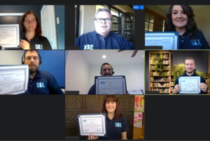
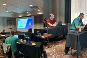
Next Page Previous Page Six Sigma Home Tools & Aids Search Handbook


1. Exploratory Data Analysis
1.3. EDA Techniques
1.3.5. Quantitative Techniques

1.3.5.16.

Kolmogorov-Smirnov Goodness-of-Fit Test

Purpose:
Test for Distributional Adequacy
The Kolmogorov-Smirnov test (Chakravart, Laha, and Roy, 1967) is used to decide if a sample comes from a population with a specific distribution.

The Kolmogorov-Smirnov (K-S) test is based on the empirical distribution function (ECDF). Given N ordered data points Y1, Y2, ..., YN, the ECDF is defined as

where n(i) is the number of points less than Yi and the Yi are ordered from smallest to largest value. This is a step function that increases by 1/N at the value of each ordered data point.

The graph below is a plot of the empirical distribution function with a normal cumulative distribution function for 100 normal random numbers. The K-S test is based on the maximum distance between these two curves.

Characteristics and Limitations of the K-S Test An attractive feature of this test is that the distribution of the K-S test statistic itself does not depend on the underlying cumulative distribution function being tested. Another advantage is that it is an exact test (the chi-square goodness-of-fit test depends on an adequate sample size for the approximations to be valid). Despite these advantages, the K-S test has several important limitations:
  1. It only applies to continuous distributions.
  2. It tends to be more sensitive near the center of the distribution than at the tails.
  3. Perhaps the most serious limitation is that the distribution must be fully specified. That is, if location, scale, and shape parameters are estimated from the data, the critical region of the K-S test is no longer valid. It typically must be determined by simulation.

Due to limitations 2 and 3 above, many analysts prefer to use the Anderson-Darling goodness-of-fit test. However, the Anderson-Darling test is only available for a few specific distributions.

Definition The Kolmogorov-Smirnov test is defined by:

H0: The data follow a specified distribution
Ha: The data do not follow the specified distribution
Test Statistic: The Kolmogorov-Smirnov test statistic is defined as
where F is the theoretical cumulative distribution of the distribution being tested which must be a continuous distribution (i.e., no discrete distributions such as the binomial or Poisson), and it must be fully specified (i.e., the location, scale, and shape parameters cannot be estimated from the data).
Significance Level: .
Critical Values: The hypothesis regarding the distributional form is rejected if the test statistic, D, is greater than the critical value obtained from a table. There are several variations of these tables in the literature that use somewhat different scalings for the K-S test statistic and critical regions. These alternative formulations should be equivalent, but it is necessary to ensure that the test statistic is calculated in a way that is consistent with how the critical values were tabulated.

We do not provide the K-S tables in the Handbook since software programs that perform a K-S test will provide the relevant critical values.

Sample Output
Dataplot generated the following output for the Kolmogorov-Smirnov test where 1,000 random numbers were generated for a normal, double exponential, t with 3 degrees of freedom, and lognormal distributions. In all cases, the Kolmogorov-Smirnov test was applied to test for a normal distribution. The Kolmogorov-Smirnov test accepts the normality hypothesis for the case of normal data and rejects it for the double exponential, t, and lognormal data with the exception of the double exponential data being significant at the 0.01 significance level.

The normal random numbers were stored in the variable Y1, the double exponential random numbers were stored in the variable Y2, the t random numbers were stored in the variable Y3, and the lognormal random numbers were stored in the variable Y4.

       *********************************************************
       **  normal Kolmogorov-Smirnov goodness of fit test y1  **
       *********************************************************
  
  
                   KOLMOGOROV-SMIRNOV GOODNESS-OF-FIT TEST
  
 NULL HYPOTHESIS H0:      DISTRIBUTION FITS THE DATA
 ALTERNATE HYPOTHESIS HA: DISTRIBUTION DOES NOT FIT THE DATA
 DISTRIBUTION:            NORMAL
    NUMBER OF OBSERVATIONS      =     1000
  
 TEST:
 KOLMOGOROV-SMIRNOV TEST STATISTIC     =   0.2414924E-01
  
    ALPHA LEVEL         CUTOFF              CONCLUSION
            10%        0.03858               ACCEPT H0
             5%        0.04301               ACCEPT H0
             1%        0.05155               ACCEPT H0
  
       *********************************************************
       **  normal Kolmogorov-Smirnov goodness of fit test y2  **
       *********************************************************
  
  
                   KOLMOGOROV-SMIRNOV GOODNESS-OF-FIT TEST
  
 NULL HYPOTHESIS H0:      DISTRIBUTION FITS THE DATA
 ALTERNATE HYPOTHESIS HA: DISTRIBUTION DOES NOT FIT THE DATA
 DISTRIBUTION:            NORMAL
    NUMBER OF OBSERVATIONS      =     1000
  
 TEST:
 KOLMOGOROV-SMIRNOV TEST STATISTIC     =   0.5140864E-01
  
    ALPHA LEVEL         CUTOFF              CONCLUSION
            10%        0.03858               REJECT H0
             5%        0.04301               REJECT H0
             1%        0.05155               ACCEPT H0
  
       *********************************************************
       **  normal Kolmogorov-Smirnov goodness of fit test y3  **
       *********************************************************
  
  
                   KOLMOGOROV-SMIRNOV GOODNESS-OF-FIT TEST
  
 NULL HYPOTHESIS H0:      DISTRIBUTION FITS THE DATA
 ALTERNATE HYPOTHESIS HA: DISTRIBUTION DOES NOT FIT THE DATA
 DISTRIBUTION:            NORMAL
    NUMBER OF OBSERVATIONS      =     1000
  
 TEST:
 KOLMOGOROV-SMIRNOV TEST STATISTIC     =   0.6119353E-01
  
    ALPHA LEVEL         CUTOFF              CONCLUSION
            10%        0.03858               REJECT H0
             5%        0.04301               REJECT H0
             1%        0.05155               REJECT H0
  
       *********************************************************
       **  normal Kolmogorov-Smirnov goodness of fit test y4  **
       *********************************************************
  
  
                   KOLMOGOROV-SMIRNOV GOODNESS-OF-FIT TEST
  
 NULL HYPOTHESIS H0:      DISTRIBUTION FITS THE DATA
 ALTERNATE HYPOTHESIS HA: DISTRIBUTION DOES NOT FIT THE DATA
 DISTRIBUTION:            NORMAL
    NUMBER OF OBSERVATIONS      =     1000
  
 TEST:
 KOLMOGOROV-SMIRNOV TEST STATISTIC     =   0.5354889
  
    ALPHA LEVEL         CUTOFF              CONCLUSION
            10%        0.03858               REJECT H0
             5%        0.04301               REJECT H0
             1%        0.05155               REJECT H0
      
Questions The Kolmogorov-Smirnov test can be used to answer the following types of questions:
  • Are the data from a normal distribution?
  • Are the data from a log-normal distribution?
  • Are the data from a Weibull distribution?
  • Are the data from an exponential distribution?
  • Are the data from a logistic distribution?
Importance Many statistical tests and procedures are based on specific distributional assumptions. The assumption of normality is particularly common in classical statistical tests. Much reliability modeling is based on the assumption that the data follow a Weibull distribution.

There are many non-parametric and robust techniques that are not based on strong distributional assumptions. By non-parametric, we mean a technique, such as the sign test, that is not based on a specific distributional assumption. By robust, we mean a statistical technique that performs well under a wide range of distributional assumptions. However, techniques based on specific distributional assumptions are in general more powerful than these non-parametric and robust techniques. By power, we mean the ability to detect a difference when that difference actually exists. Therefore, if the distributional assumptions can be confirmed, the parametric techniques are generally preferred.

If you are using a technique that makes a normality (or some other type of distributional) assumption, it is important to confirm that this assumption is in fact justified. If it is, the more powerful parametric techniques can be used. If the distributional assumption is not justified, using a non-parametric or robust technique may be required.

Related Techniques Anderson-Darling goodness-of-fit Test
Chi-Square goodness-of-fit Test
Shapiro-Wilk Normality Test
Probability Plots
Probability Plot Correlation Coefficient Plot
Case Study Airplane glass failure times data
Software Some general purpose statistical software programs, including Dataplot, support the Kolmogorov-Smirnov goodness-of-fit test, at least for some of the more common distributions.
Six Sigma Home Tools & Aids Search Handbook Previous Page Next Page